Article

Seasonal Length–Weight Relationships of European Sea Bass (Dicentrarchus labrax) in Two Aquaculture Production Systems

by
Carlos Orduna
1,2,
Ilaria de Meo
1,
Amadora Rodríguez-Ruiz
2,
Juan Ramón Cid-Quintero
1 and
Lourdes Encina
2,*
1
EcoFishUS Research S.L.L., Prof. García-González 6, 41012 Seville, Spain
2
Department of Vegetal Biology and Ecology, University of Seville, Prof. García-González 6, 41012 Seville, Spain
*
Author to whom correspondence should be addressed.
Fishes 2023, 8(5), 227; https://doi.org/10.3390/fishes8050227
Submission received: 30 March 2023 / Revised: 20 April 2023 / Accepted: 24 April 2023 / Published: 25 April 2023
(This article belongs to the Special Issue Development of Sustainable Aquaculture Production)

Abstract

:
Different non-intrusive methods have been developed to estimate fish biomass, which is a determinant factor for aquaculture farming management. Length–weight conversion is a crucial parameter for accurate biomass estimation. However, the potential environmental and seasonal variations in fish length–weight relationships are rarely considered. In this study, we examined seasonal variation in length–weight relationships for European sea bass (Dicentrarchus labrax) from two farming systems subject to different salinity and temperature conditions: inland ponds and offshore cages. The results showed significant differences in intercept and slope between the two types of facilities studied, as well as between the same seasons for both facilities. This highlights the need to use specific length–weight equations to obtain accurate biomass estimation based on fish length data.
Key Contribution: This study provides insights into the relevance of applying specific length–weight relationships to estimate biomass in aquaculture.

1. Introduction

Aquaculture is already a very important industry worldwide. With its rapid development and an average annual projected growth rate of 4.5% from 2010 to 2030, aquaculture currently surpasses extractive fishing in terms of tons produced, and more researchers are paying attention to this sector [1,2,3,4,5]. Efficient, precise, and intelligent aquaculture is the future development direction for this industry [3,4]. In this sense, monitoring fish production in aquaculture farms is essential for informed decision making and effective management. Accurate biometric, behavioral, density, and biomass data from farmed fish are crucial, especially in optimizing feed usage, which is a primary factor in determining efficiency and cost [2,6,7,8,9,10,11].
Fish biomass is usually estimated from the total number of fish counted in a pond or cage multiplied by the average weight of a fish sample [12]. Capture-dependent methods are occasionally used to know the length and weight of the farmed fish, but the inaccuracy of the results, along with the stress and the potential increase in fish mortality, has led researchers to develop new non-intrusive estimation methods [5,13,14,15]. In this sense, two techniques stand out in terms of remotely estimating the length and weight of fish in offshore aquaculture. The first is hydroacoustics, which is a widely used technique for fish detection in all kinds of aquatic environments [16,17,18,19]. This technology establishes a relationship between the intensity of the sound backscattering from fish, which is known as target strength (TS dB), and fish variables such as length or weight [20,21]. Specific TS–length equations for most of the farmed fish species have been developed, such as Atlantic salmon (Salmo salar), brown trout (Salmo trutta), perch (Perca fluviatilis), carp (Cyprinus carpio), gilt-head seabream (Sparus aurata), or sea bass (Dicentrarchus labrax) [22,23,24]. These equations allow us to use hydroacoustics to know the size of fish in a non-intrusive way. The second approach involves computer vision, which is rapidly developing as a system for obtaining fish measurements without any kind of manipulation, using stereo vision underwater cameras. This technology uses images to measure the fish size in aquaculture facilities through computer image analysis [3,12,25,26,27,28,29]. These two techniques have proven to be a good adjustment in fish size measures, but both usually need to use a previously calculated length–weight relationship to provide weight estimates from TS or stereoscopic images [11,30]. This length–weight relationship can vary with fish growth rate, due to different external or intrinsic factors [31].
The European sea bass represents one of the most important farmed fish species in southern Europe [32]. However, the potential effects of seasonal variation on length–weight equations and their implication for biomass estimation are largely unexplored. Water temperature and its significant seasonal differences are critical external factors that affect most biochemical and physiological processes in aquatic organisms, resulting in one of the most important environmental–physical factors. Increasing water temperature has a significant influence on fish growth, determining higher food intake and growth rates within the non-stressful thermal range for each species [33,34,35,36,37,38,39]. In this sense, adult sea bass species migrate to estuaries and coastal lagoons for spawning, where larvae can find optimal growth conditions and plankton prey due to the early warming of these shallow waters in spring [40]. Variation in salinity is a disturbing factor influencing the metabolism and growth of the European sea bass. Despite being a euryhaline fish, acute changes in water salinity can cause complex metabolic changes in sea bass. On the one hand, a decrease in salinity suggests a reduction in the costs associated with osmoregulation. However, salinity changes in the environment involve more than just osmoregulation costs. The gills are the main osmoregulation organ, but because of their involvement in respiration, they are at the same time the main site of water and ion leakage. Thus, as osmoregulatory costs are linked to metabolic activity through ventilation, the portion of energy necessary to compensate for the ventilation-related osmotic and ionic loss will increase, as fish metabolic expenditure rises [37,40,41,42,43,44,45,46]. Dissolved oxygen is another crucial factor for fish survival and growth in aquaculture farms. However, significant inputs of nitrogen and phosphorus due to the decomposition of uneaten feed, feces, and metabolic excretion by cultured animals can lead to substantial variation in oxygen levels. This leads to the production of oxygen by photosynthetic organisms. Furthermore, substantial amounts of oxygen are consumed in plankton and fish respiration. Therefore, dissolved oxygen concentration is a parameter closely monitored in aquaculture farms, as sudden drops in its concentration, especially at night, could result in significant fish mortality rates [35,36,40,47,48].
The aim of this study is to compare the seasonal length–weight relationships of sea bass (Dicentrarchus labrax) between two farming systems presenting different environmental conditions, to assess the benefits of using specific equations for each facility and season of the year.

2. Materials and Methods
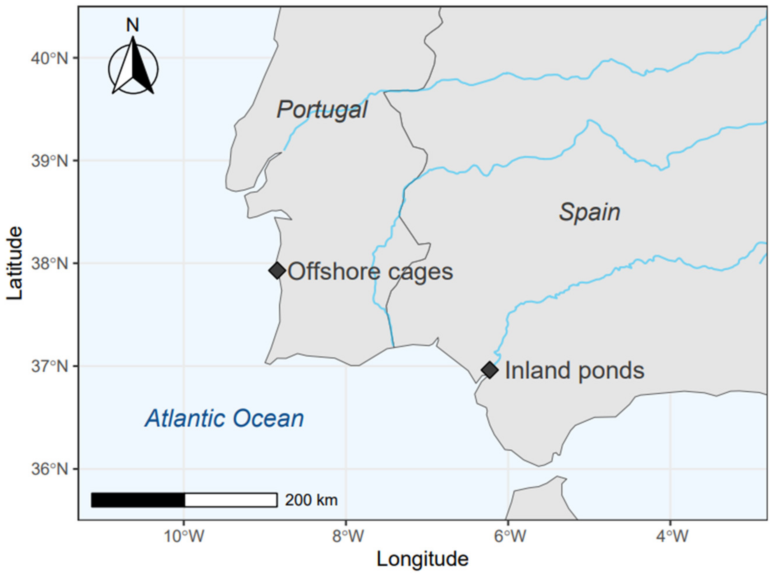
2.1. Samplings

Two different sea bass farming facilities were selected for this study (Figure 1). The first one was located in the Guadalquivir River estuary, with brackish water, in Seville, Spain. This farm system was based on rectangular inland ponds, with a surface area of 2.700 m2 and a volume of 3150 m3. The second farming facility was in the Atlantic Ocean, in the Setúbal district, Portugal. This farm consisted of cylindrical offshore cages, of an approximate volume of 6.500 m3. In both cases, the fish farm managers set the seeding and management of the facilities aiming at obtaining a density of around 5 fish/m3. Moreover, fish were fed until they were satiated during the whole breeding process. Samples were obtained seasonally for one year. About 200 sea bass were measured for each sampling. Fish were measured in the field for standard length (SL) to the nearest millimeter, and weighed (W, wet weight) to the nearest gram. All the specimens were measured during the harvest process before sales, with all of them being approximately the same age. Daily records of temperature and salinity were provided by the managers of the facilities, except for offshore salinity due to its low variation. Previous studies monitoring water quality in the study area where the offshore facilities were located reported average salinity values of 36 PSU, with little inter- and intra-annual variability [49,50]. Thus, we considered this parameter as constant.

2.2. Data Analysis

All statistical analyses were conducted in the statistical package R [51]. The power function W = aSLb is commonly used to predict fish weight from the fish length, where W is the total body weight of the fish in grams, SL is the standard length in millimeters, a is the regression intercept, and b is the regression slope. This length–weight model was transformed into a linear model by applying a log10 transformation to both sides, resulting in the equation log(W) = log(a) + b log(SL). Using the logarithmic form of the equation, length–weight relationships were estimated for each season in each farming facility. The values of the regression slope indicate isometric (b = 3) or allometric (positive if b > 3, negative if b < 3) growth. In order to investigate the seasonal growth pattern in each farming facility, a Student’s t-test was performed to evaluate if the mean b value was significantly different from 3 and to identify the type of growth. Moreover, significant differences in the intercept and slope were analyzed among seasons within each facility using analysis of covariance (ANCOVA) with log(W) as the response variable, log(L) as the continuous covariate, and “season” as the categorical variable. Seasonal differences were also tested in length–weight relationships between facilities by fitting an ANCOVA separately for each season with “facility” as the categorical variable. The assumptions of normality and homoscedasticity were verified through the inspection of the quantile–quantile plot and the residual-against-fit plot, respectively.
In order to verify the actual differences that may result from using different equations, a practical case was performed to estimate fish biomass through their application. Length–frequency distribution was simulated for an inland pond and an offshore cage of the two studied farming facilities. Fish length–frequency distribution was obtained by simulating random length values for each size interval of the target strength (TS) frequency distribution from previously collected acoustic data, specifying the length range and the number of individuals for each range [5,10]. The predictions of individual weight values and confidence intervals given the length values were achieved by fitting the specific regression for each season using the predict function from the “stats” R package. The predicted weights were then back-transformed to the original scale and corrected for bias using the logbtcf function from the “FSA” R package [52].

3. Results

The seasonal sea bass length–weight regressions of the two studied farming facilities are shown in Table 1 and Figure 2. The r2 values ranged from 0.844 for the inland farm in winter to 0.957 for the offshore farm in autumn and were all highly significant (p ≤ 0.001).
Sea bass presented different growth types within each facility. Fish from the inland facility showed isometric growth (b = 3) in summer and autumn and negative allometric growth (b < 3) in winter and spring. On the other hand, sea bass from the offshore facility presented isometric growth (b = 3) in winter, negative allometric growth (b < 3) in summer, and positive allometric growth (b > 3) in spring and autumn (Table 1).
Significant differences were found in the intercept and slope among seasons for the inland (ANCOVA, F12.791; p < 0.001) and offshore (ANCOVA, F13.414; p < 0.001) facilities.
Seasonal differences test in the length–weight relationships between facilities for each season also showed significant differences for all of them: autumn (ANCOVA, F5.772; p < 0.001), spring (ANCOVA, F30.658; p < 0.001), summer (ANCOVA, F15.642; p < 0.001) and winter (ANCOVA, F12.881; p < 0.001).
The results of the total biomass simulation for two cases of both studied facilities, i.e., an inland pond and an offshore cage, are shown in Figure 3.

4. Discussion

In this study, we compared two different aquaculture facilities located only 250 km apart but presenting significant differences in water temperature and salinity. This is mainly because the offshore cages are situated in the ocean, while the ponds are located inland, specifically in an estuary area.
In aquaculture facilities, such as those selected for this study, food and oxygen concentration in the water are not limiting factors. In offshore cages, automatic feeders and a camera system controlled by an operator stop feeding when leftover food is detected. While this system does not allow for the precise dosing of feed and results in significant feed waste, it ensures that the fish are fed until they are fully satiated. In inland ponds, fish have feeders that release food on demand when fish approach the feeding area and activate a floating ball. Workers also provide extra feed during times of high demand, ensuring that fish are fully satiated, although with little precision and significant waste. Moreover, the oxygen concentration was monitored in both types of facilities studied, with particular attention paid to the inland ponds, where compressed oxygen systems were available to inject oxygen into the ponds in case of a sudden drop that could have caused fish mortality.
Temperature and salinity are the two most influential environmental factors on the growth and metabolism of farmed fish since they are hard to control [34,35,36,53,54]. In this regard, the water in offshore cages primarily consisted of coastal water from the Atlantic Ocean that was constantly renewed through the cage’s net wall. As a result, the annual average temperature remained around 15.9 °C with a low fluctuation of 7.6 °C, and the salinity remained constant at around 36 ppt (Figure 4), which is similar to the natural habitat of these fish. By contrast, estuaries are complex aquatic systems where river and sea dynamics interact, creating unique conditions that evolve in space and time across various scales [55]. This interaction varies continuously throughout the estuary with each tidal cycle, neap, and spring tides, and it is drastically altered during brief periods associated with the occurrence of river floods [56]. This environmental variation, combined with the fact that inland ponds have much lower water renewal rates (just through a channel that runs across the pond) and much shallower depths, can cause great fluctuations in temperature and salinity, as they lack the buffering effect of the ocean, even though the climates of both facilities are similar. In inland ponds, water temperature ranged from 10 °C in winter to 30 °C in summer, with an average temperature of 20.7 °C, while salinity averaged 18 ppt and reached a maximum of 25 ppt in autumn (Figure 4), always being lower than in offshore cages. Previous experimental studies suggest that the preferred temperatures for this species range between 20 and 25 °C [37,40]. Under experimental conditions, the sea bass growth rate increased with increasing salinity, reaching a maximum at 33 ppt [47]. However, acute changes in water salinity can rapidly increase fish metabolic rate due to osmoregulation and respiration [37,40,57]. In addition, sea bass presented different growth types within each facility, showing the important effect of seasonal variation on fish growth patterns. Positive allometric values, defined as cases in which fish became stouter with increasing body length, were only observed for offshore cages in spring and autumn, while fish from inland ponds presented isometric or negative allometric growth. Fish growth in offshore cages may be favored by relatively stable water temperatures around the preferred range and constant salinity conditions. Environmental conditions experienced in early life can also play an important role in the morphology and growth trajectories of sea bass [58], suggesting that seeding season might be an important factor to consider in farm management.
Assuming that temperature and salinity variations are responsible for the observed differences in the length–weight relationship of fish among different facilities and seasons, it is crucial to account for such variations when estimating biomass based on length. In this regard, the practical case presented in Figure 3 shows the variations in the estimated biomass for a cultivation unit in the two kinds of studied facilities. The data reveal significant differences, with variations reaching up to 31.5% between winter and autumn in inland ponds, and 28.5% in offshore cages between winter and spring, which are the seasons that exhibit the greatest differences, respectively. These substantial differences should be taken into consideration when estimating fish biomass. Increasingly precise methods are being developed to remotely estimate the length of fish, and the same precision should be the goal for the length–weight conversion, as the total biomass is the estimated value that really matters to fish farmers for the management of their companies.

5. Conclusions

Our research highlights the need to use specific length–weight equations for aquaculture facilities that take into account seasonal environmental variations. Many studies aim to establish the most accurate possible length estimates of fish using remote detection methods, such as techniques involving digital imaging or hydroacoustics [59,60,61,62]. Avoiding capture-dependent methods that cause high levels of stress to fish can prevent potential increases in mortality [5,13,14,15]. However, it should not be assumed that the length–weight conversion is a minor issue, as the selection of a specific equation can cause significant variations in biomass estimates. This is particularly important in aquaculture, as having accurate estimates of density and biomass in these farms allows managers to obtain important information for optimizing feed dosage [5,6] (a major production cost for these companies) or managing stocks and sales, all of which are crucial aspects for the sector.

Author Contributions

Conceptualization, C.O., L.E. and A.R.-R.; methodology, C.O. and J.R.C.-Q.; software, I.d.M.; validation, L.E. and A.R.-R.; writing—original draft preparation, C.O. and I.d.M.; writing—review and editing, L.E. and A.R.-R.; project administration, C.O. and J.R.C.-Q.; funding acquisition, C.O. and J.R.C.-Q. All authors have read and agreed to the published version of the manuscript.

Funding

This study has been funded by the own funds of EcoFishUS Research, a spin-off of the University of Seville dedicated to knowledge transfer, and by the University of Seville through the Research and Transfer Plan, with a doctoral scholarship in collaboration with companies.

Institutional Review Board Statement

Our study involved only fish that were caught and immediately sacrificed for the purpose of sale. We did not work with live animals in any way. As part of our research, we took measurements of the fish that had already been sacrificed for commercial purposes. Therefore, we believe that Ethics Committee or Institutional Review Board approval is not required for our manuscript.

Data Availability Statement

Restrictions apply to the availability of these data. Data was obtained from two private fish production companies and are available on request from the corresponding author with the permission of the companies.

Conflicts of Interest

The authors declare no conflict of interest.

References

  1. Brugére, C.; Ridler, N. Global Aquaculture Outlook in the next Decades: An Analysis of National Aquaculture Production Forecasts to 2030. FAO Fish. Circ. 2004, 1001, 47. [Google Scholar]
  2. Zhou, C.; Xu, D.; Lin, K.; Sun, C.; Yang, X. Intelligent Feeding Control Methods in Aquaculture with an Emphasis on Fish: A Review. Rev. Aquac. 2018, 10, 975–993. [Google Scholar] [CrossRef]
  3. An, D.; Hao, J.; Wei, Y.; Wang, Y.; Yu, X. Application of Computer Vision in Fish Intelligent Feeding System—A Review. Aquac. Res. 2021, 52, 423–437. [Google Scholar] [CrossRef]
  4. Goldburg, R.; Naylor, R. Future Seascapes, Fishing, and Fish Farming. Front. Ecol. Environ. 2005, 3, 21–28. [Google Scholar] [CrossRef]
  5. Orduna, C.; Encina, L.; Rodríguez-Ruiz, A.; Rodríguez-Sánchez, V. Testing of New Sampling Methods and Estimation of Size Structure of Sea Bass (Dicentrarchus labrax) in Aquaculture Farms Using Horizontal Hydroacoustics. Aquaculture 2021, 545, 737242. [Google Scholar] [CrossRef]
  6. Soliveres, E.; Puig, V.; Perez-arjona, I. Acoustical Biomass Estimation Results in Mediterranean Aquaculture Sea Cages. In Proceedings of the UA2014—2nd International Conference and Exhibition on Underwater Acoustics, Rhodes, Greece, 22–27 June 2014; pp. 1423–1428. [Google Scholar]
  7. Pérez, J.M.; Sarasa, M.; Moço, G.; Granados, J.E.; Crampe, J.P.; Serrano, E.; Maurino, L.; Meneguz, P.G.; Afonso, A.; Alpizar-Jara, R. The Effect of Data Analysis Strategies in Density Estimation of Mountain Ungulates Using Distance Sampling. Ital. J. Zool. 2015, 82, 262–270. [Google Scholar] [CrossRef]
  8. Hofmeester, T.R.; Rowcliffe, J.M.; Jansen, P.A. A Simple Method for Estimating the Effective Detection Distance of Camera Traps. Remote Sens. Ecol. Conserv. 2016, 3, 81–89. [Google Scholar] [CrossRef]
  9. Føre, M.; Alver, M.; Alfredsen, J.A.; Marafioti, G.; Senneset, G.; Birkevold, J.; Willumsen, F.V.; Lange, G.; Espmark, Å.; Terjesen, B.F. Modelling Growth Performance and Feeding Behaviour of Atlantic Salmon (Salmo salar L.) in Commercial-Size Aquaculture Net Pens: Model Details and Validation through Full-Scale Experiments. Aquaculture 2016, 464, 268–278. [Google Scholar] [CrossRef]
  10. Orduna, C.; Encina, L.; Rodríguez-Ruiz, A.; Rodríguez-Sánchez, V. Hydroacoustics for Density and Biomass Estimations in Aquaculture Ponds. Aquaculture 2021, 545, 737240. [Google Scholar] [CrossRef]
  11. Rodríguez-Sánchez, V.; Rodríguez-Ruiz, A.; Pérez-Arjona, I.; Encina-Encina, L. Horizontal Target Strength-Size Conversion Equations for Sea Bass and Gilt-Head Bream. Aquaculture 2018, 490, 178–184. [Google Scholar] [CrossRef]
  12. Harvey, E.; Cappo, M.; Shortis, M.; Robson, S.; Buchanan, J.; Speare, P. The Accuracy and Precision of Underwater Measurements of Length and Maximum Body Depth of Southern Bluefin Tuna (Thunnus maccoyii) with a Stereo-Video Camera System. Fish. Res. 2003, 63, 315–326. [Google Scholar] [CrossRef]
  13. Espinosa, V.; Ramis, J.; Alba, J. Evaluación de La Sonda Ultrasónica EY-500 de Simrad Para El Control de Explotaciones de Dorada Sparus Auratus Linnaeus, 1758. Bol. Inst. Esp. Oceanogr. 2002, 18, 15–19. [Google Scholar]
  14. Conti, S.G.; Roux, P.; Fauvel, C.; Maurer, B.D.; Demer, D.A. Acoustical Monitoring of Fish Density, Behavior, and Growth Rate in a Tank. Aquaculture 2006, 251, 314–323. [Google Scholar] [CrossRef]
  15. The Humane Society of the United States. The Welfare of Animals in the Aquaculture Industry. Hsus Rep. 2008, 5, 24. [Google Scholar]
  16. Godlewska, M.; Frouzova, J.; Kubecka, J.; Wiśniewolski, W.; Szlakowski, J. Comparison of Hydroacoustic Estimates with Fish Census in Shallow Malta Reservoir—Which TS/L Regression to Use in Horizontal Beam Applications? Fish. Res. 2012, 123, 90–97. [Google Scholar] [CrossRef]
  17. Dennerline, D.E.; Jennings, C.A.; Degan, D.J. Relationships between Hydroacoustic Derived Density and Gill Net Catch: Implications for Fish Assessments. Fish. Res. 2012, 123, 78–89. [Google Scholar] [CrossRef]
  18. Greenstreet, S.P.R.; Holland, G.J.; Guirey, E.J.; Armstrong, E.; Fraser, H.M.; Gibb, I.M. Combining Hydroacoustic Seabed Survey and Grab Sampling Techniques to Assess “Local” Sandeel Population Abundance. ICES J. Mar. Sci. 2010, 67, 971–984. [Google Scholar] [CrossRef]
  19. Koliada, I.; Balk, H.; Tušer, M.; Ptáček, L.; Kubečka, J. Limitations of Target Detection in Horizontal Acoustic Surveys of Extremely Shallow Water Bodies. Fish. Res. 2019, 218, 94–104. [Google Scholar] [CrossRef]
  20. Simmonds, J.; MacLennan, D. Fisheries Acoustics: Theory and Practice; Blackwell Science Ltd.: Hoboken, NJ, USA, 2005; ISBN 978-0-632-05994-2. [Google Scholar]
  21. Rodríguez-Sánchez, V.; Encina-Encina, L.; Rodríguez-Ruiz, A.; Sánchez-Carmona, R. Do Close Range Measurements Affect the Target Strength (TS) of Fish in Horizontal Beaming Hydroacoustics? Fish. Res. 2016, 173, 4–10. [Google Scholar] [CrossRef]
  22. Lilja, J.; Marjomäki, T.J.; Riikonen, R.; Jurvelius, J. Side-Aspect Target Strength of Atlantic Salmon (Salmo salar), Brown Trout (Salmo trutta), Whitefish (Coregonus lavaretus), and Pike (Esox lucius). Aquat. Living Resour. 2000, 13, 355–360. [Google Scholar] [CrossRef]
  23. Frouzova, J.; Kubecka, J.; Balk, H.; Frouz, J. Target Strength of Some European Fish Species and Its Dependence on Fish Body Parameters. Fish. Res. 2005, 75, 86–96. [Google Scholar] [CrossRef]
  24. Rodríguez-Sánchez, V.; Encina-Encina, L.; Rodríguez-Ruiz, A.; Monteoliva, A.; Sánchez-Carmona, R. Horizontal Target Strength of Cyprinus Carpio Using 200 kHz and 430 kHz Split-Beam Systems. Fish. Res. 2016, 174, 136–142. [Google Scholar] [CrossRef]
  25. Harvey, E.; Fletcher, D.; Shortis, M. Estimation of Reef Fish Length by Divers and by Stereo-Video. Fish. Res. 2002, 57, 255–265. [Google Scholar] [CrossRef]
  26. Costa, C.; Loy, A.; Cataudella, S.; Davis, D.; Scardi, M. Extracting Fish Size Using Dual Underwater Cameras. Aquac. Eng. 2006, 35, 218–227. [Google Scholar] [CrossRef]
  27. De La Gandara, F.; Espinosa, V. Estimación Del Número y La Biomasa de Individuos Por Métodos Acústicos En El Cultivo Del Atún Rojo (Thunnus thynnus). Collect. Vol. Sci. Pap. ICCAT 2012, 68, 276–283. [Google Scholar]
  28. Islamadina, R.; Pramita, N.; Arnia, F.; Munadi, K. Estimating Fish Weight Based on Visual Captured. In Proceedings of the 2018 International Conference on Information and Communications Technology (ICOIACT), Yogyakarta, Indonesia, 6–7 March 2018; pp. 366–372. [Google Scholar] [CrossRef]
  29. Muñoz-Benavent, P.; Andreu-García, G.; Valiente-González, J.M.; Atienza-Vanacloig, V.; Puig-Pons, V.; Espinosa, V. Enhanced Fish Bending Model for Automatic Tuna Sizing Using Computer Vision. Comput. Electron. Agric. 2018, 150, 52–61. [Google Scholar] [CrossRef]
  30. Martinez-De Dios, J.R.; Serna, C.; Ollero, A. Computer Vision and Robotics Techniques in Fish Farms. Robotica 2003, 21, 233–243. [Google Scholar] [CrossRef]
  31. Person-Le Ruyet, J.; Mahé, K.; Le Bayon, N.; Le Delliou, H. Effects of Temperature on Growth and Metabolism in a Mediterranean Population of European Sea Bass, Dicentrarchus labrax. Aquaculture 2004, 237, 269–280. [Google Scholar] [CrossRef]
  32. Llorente, I.; Fernández-Polanco, J.; Baraibar-Diez, E.; Odriozola, M.D.; Bjørndal, T.; Asche, F.; Guillen, J.; Avdelas, L.; Nielsen, R.; Cozzolino, M.; et al. Assessment of the Economic Performance of the Seabream and Seabass Aquaculture Industry in the European Union. Mar. Policy 2020, 117, 103876. [Google Scholar] [CrossRef]
  33. Elliot, R. Faking Nature. Inquiry 1982, 25, 81–93. [Google Scholar] [CrossRef]
  34. Hidalgo, F.; Alliot, E.; Thebault, H. Influence of Water Temperature on Food Intake, Food Efficiency and Gross Composition of Juvenile Sea Bass, Dicentrarchus labrax. Aquaculture 1987, 64, 199–207. [Google Scholar] [CrossRef]
  35. Deane, E.E.; Woo, N.Y.S. Modulation of Fish Growth Hormone Levels by Salinity, Temperature, Pollutants and Aquaculture Related Stress: A Review. Rev. Fish Biol. Fish. 2009, 19, 97–120. [Google Scholar] [CrossRef]
  36. Besson, M.; Vandeputte, M.; van Arendonk, J.A.M.; Aubin, J.; de Boer, I.J.M.; Quillet, E.; Komen, H. Influence of Water Temperature on the Economic Value of Growth Rate in Fish Farming: The Case of Sea Bass (Dicentrarchus labrax) Cage Farming in the Mediterranean. Aquaculture 2016, 462, 47–55. [Google Scholar] [CrossRef]
  37. Claireaux, G.; Lagardère, J.P. Influence of Temperature, Oxygen and Salinity on the Metabolism of the European Sea Bass. J. Sea Res. 1999, 42, 157–168. [Google Scholar] [CrossRef]
  38. Reynolds, W.W.; Casterlin, M.E. Behavioral Thermoregulation and the “Final Preferendum” Paradigm. Integr. Comp. Biol. 1979, 19, 211–224. [Google Scholar] [CrossRef]
  39. Zanuy, S.; Carrillo, M. Annual Cycles of Growth, Feeding Rate, Gross Conversion Efficiency and Hematocrit Levels of Sea Bass (Dicentrarchus labrax L.) Adapted to Two Different Osmotic Media. Aquaculture 1985, 44, 11–25. [Google Scholar] [CrossRef]
  40. Dalla Via, J.; Villani, P.; Gasteiger, E.; Niederstätter, H. Oxygen Consumption in Sea Bass Fingerling Dicentrarchus labrax Exposed to Acute Salinity and Temperature Changes: Metabolic Basis for Maximum Stocking Density Estimations. Aquaculture 1998, 169, 303–313. [Google Scholar] [CrossRef]
  41. Von Oertzen, J.A. Influence of Steady-State and Fluctuating Salinities on the Oxygen Consumption and Activity of Some Brackish Water Shrimps and Fishes. J. Exp. Mar. Biol. Ecol. 1984, 80, 29–46. [Google Scholar] [CrossRef]
  42. Rao, G.M.M. Oxygen Consumption of Rainbow Trout (Salmo gairdneri) in Relation to Activity and Salinity. Can. J. Zool. 1968, 46, 781–786. [Google Scholar] [CrossRef]
  43. Farmer, G.J.; Beamish, F.W.H. Oxygen Consumption of Tilapia Nilotica in Relation to Swimming Speed and Salinity. J. Fish. Res. Board Canada 1969, 26, 2807–2821. [Google Scholar] [CrossRef]
  44. Boyd, C.E.; Torrans, E.L.; Tucker, C.S. Dissolved Oxygen and Aeration in Ictalurid Catfish Aquaculture. J. World Aquac. Soc. 2018, 49, 7–70. [Google Scholar] [CrossRef]
  45. Ma, Y.; Ding, W. Design of Intelligent Monitoring System for Aquaculture Water Dissolved Oxygen. In Proceedings of the 2018 IEEE 3rd Advanced Information Technology, Electronic and Automation Control Conference (IAEAC), Chongqing, China, 12–14 October 2018; pp. 414–418. [Google Scholar] [CrossRef]
  46. Li, C.; Li, Z.; Wu, J.; Zhu, L.; Yue, J. A Hybrid Model for Dissolved Oxygen Prediction in Aquaculture Based on Multi-Scale Features. Inf. Process. Agric. 2018, 5, 11–20. [Google Scholar] [CrossRef]
  47. Dendrinos, P.; Thorpe, J.P. Effects of Reduced Salinity on Growth and Body Composition in the European Bass Dicentrarchus labrax (L.). Aquaculture 1985, 49, 333–358. [Google Scholar] [CrossRef]
  48. Eroldoǧan, O.T.; Kumlu, M.; Aktaş, M. Optimum Feeding Rates for European Sea Bass Dicentrarchus labrax L. Reared in Seawater and Freshwater. Aquaculture 2004, 231, 501–515. [Google Scholar] [CrossRef]
  49. Gomes, M.; Correia, A.; Pinto, L.; Sá, C.; Brotas, V.; Mateus, M. Coastal Water Quality in an Atlantic Sea Bass Farm Site (Sines, Portugal): A First Assessment. Front. Mar. Sci. 2020, 7, 175. [Google Scholar] [CrossRef]
  50. Mosqueira, M.; Pombo, A.; Borges, C.; Brito, A.C.; Zacarias, N.; Esteves, R.; Palma, C. Potential for Coastal and Offshore Aquaculture in Portugal: Insights from Physico-Chemical and Oceanographic Conditions. Appl. Sci. 2022, 12, 2742. [Google Scholar] [CrossRef]
  51. R Core Team. R: A Language and Environment for Statistical Computing; Austria R Foundation for Statistical Computing: Vienna, Austria, 2022. [Google Scholar]
  52. Ogle, D.H.; Doll, J.C.; Wheeler, A.P.; Dinno, A. FSA: Simple Fisheries Stock Assessment Methods. 2023. Available online: https://cran.r-project.org/package=FSA (accessed on 30 March 2023).
  53. Jobling, M. The Thermal Growth Coefficient (TGC) Model of Fish Growth: A Cautionary Note. Aquac. Res. 2003, 34, 581–584. [Google Scholar] [CrossRef]
  54. Jauralde, I.; Martínez-Llorens, S.; Tomás, A.; Ballestrazzi, R.; Jover, M. A Proposal for Modelling the Thermal-Unit Growth Coefficient and Feed Conversion Ratio as Functions of Feeding Rate for Gilthead Sea Bream (Sparus aurata, L.) in Summer Conditions. Aquac. Res. 2013, 44, 242–253. [Google Scholar] [CrossRef]
  55. Bramato, S.; Losada, M.A.; Contreras, E.; Polo, M. An Integrated Database Manager to Forecast Estuarine Dynamics and Water Quality in the Guadalquivir River (Spain). River Flow 2010, 2, 1415–1420. [Google Scholar]
  56. Contreras, E.; Polo, M.J. Measurement Frequency and Sampling Spatial Domains Required to Characterize Turbidity and Salinity Events in the Guadalquivir Estuary (Spain). Nat. Hazards Earth Syst. Sci. 2012, 12, 2581–2589. [Google Scholar] [CrossRef]
  57. Precht, H.; Christophersen, J.; Hensel, H. Temperatur Und Leben; Springer: Berlin/Heidelberg, Germany, 1955; p. 514. [Google Scholar]
  58. Georgakopoulou, E.; Sfakianakis, D.G.; Kouttouki, S.; Divanach, P.; Kentouri, M.; Koumoundouros, G. The Influence of Temperature during Early Life on Phenotypic Expression at Later Ontogenetic Stages in Sea Bass. J. Fish Biol. 2007, 70, 278–291. [Google Scholar] [CrossRef]
  59. Boswell, K.M.; Wilson, M.P.; Wilson, C.A. Hydroacoustics as a Tool for Assessing Fish Biomass and Distribution Associated with Discrete Habitats in a Louisiana Estuary. Estuaries Coasts 2007, 30, 607–617. [Google Scholar] [CrossRef]
  60. Álvarez-Ellacuría, A.; Palmer, M.; Catalán, I.A.; Lisani, J.L. Image-Based, Unsupervised Estimation of Fish Size from Commercial Landings Using Deep Learning. ICES J. Mar. Sci. 2020, 77, 1330–1339. [Google Scholar] [CrossRef]
  61. Hsieh, C.L.; Chang, H.Y.; Chen, F.H.; Liou, J.H.; Chang, S.K.; Lin, T. Te A Simple and Effective Digital Imaging Approach for Tuna Fish Length Measurement Compatible with Fishing Operations. Comput. Electron. Agric. 2011, 75, 44–51. [Google Scholar] [CrossRef]
  62. Shi, C.; Wang, Q.; He, X.; Zhang, X.; Li, D. An Automatic Method of Fish Length Estimation Using Underwater Stereo System Based on LabVIEW. Comput. Electron. Agric. 2020, 173, 105419. [Google Scholar] [CrossRef]
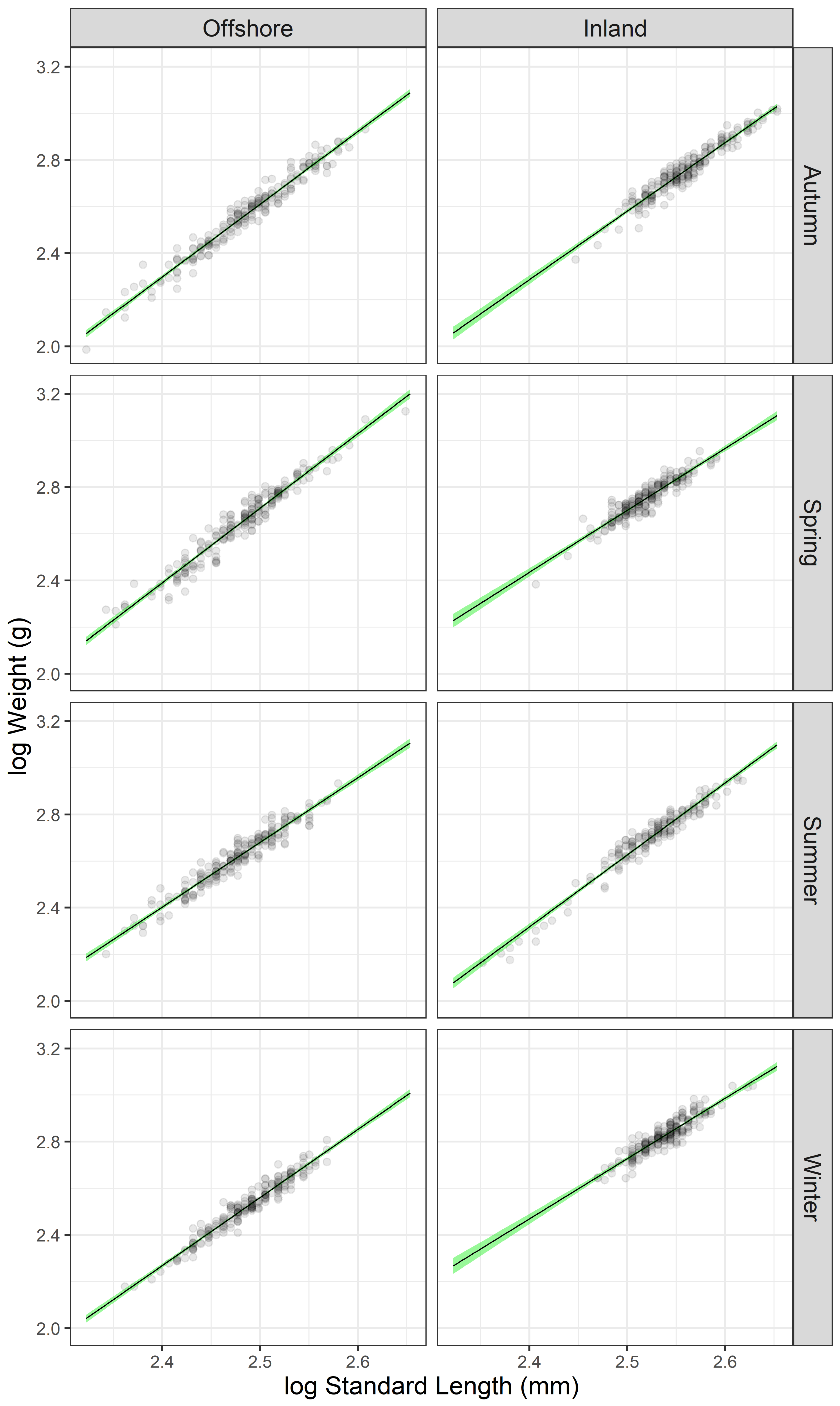
Figure 1. Location of the sea bass farming facilities.
Fishes 08 00227 g001
Figure 2. Seasonal seas bass length–weight relationship for the offshore and inland farms. Green area indicates the 95% confidence interval.
Fishes 08 00227 g002
Figure 3. Biomass simulation for the two studied facilities: an inland pond (a) and an offshore cage (b). Error bars represent the estimated 95% confidence intervals.
Fishes 08 00227 g003
Figure 4. Daily temperature (a) and salinity (b) variation in the two studied locations: inland ponds (red lines) and offshore cages (blue lines).
Fishes 08 00227 g004
Table 1. Seasonal seas bass length–weight regressions for the offshore and inland farms.
FacilitySeasonnSL (mm)W (g)log(a)95% C.I. log(a)b95% C.I. br2Growth
OffshoreWinter196308 ± 28345 ± 92−4.740−4.990; −4.4902.9202.820–3.0210.944 *Isometric
OffshoreSpring197303 ± 35470 ± 179−5.292−5.564; −5.0193.2013.091–3.3110.944 *Allometric (+)
OffshoreSummer200300 ± 30426 ± 120−4.262−4.528; −3.9962.7772.700–2.8840.929 *Allometric (−)
OffshoreAutumn197309 ± 37397 ± 148−5.193−5.424; −4.9613.1213.028–3.2140.957 *Allometric (+)
InlandWinter198346 ± 22678 ± 120−3.736−4.132; −3.3402.5852.429–2.7420.844 *Allometric (−)
InlandSpring200331 ± 22575 ± 107−3.940−4.305; −3.5762.6562.512–2.8010.868 *Allometric (−)
InlandSummer166336 ± 34526 ± 149−5.087−5.366; −4.8093.0852.975–3.1960.949 *Isometric
InlandAutumn200364 ± 32587 ± 157−4.763−5.057; −4.4702.9372.823–3.0520.928 *Isometric
Number of specimens (n); mean ± standard deviation; standard length (SL) and weight (W); intercept of regression line (a); slope of regression line (b); confidence interval (C.I.); regression coefficient (r2); * significant p ≤ 0.001.
Disclaimer/Publisher’s Note: The statements, opinions and data contained in all publications are solely those of the individual author(s) and contributor(s) and not of MDPI and/or the editor(s). MDPI and/or the editor(s) disclaim responsibility for any injury to people or property resulting from any ideas, methods, instructions or products referred to in the content.

